Graphics Gallery Tutorial

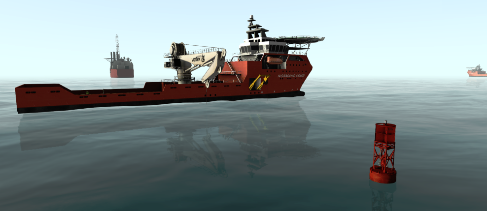
In this tutorial, you will learn the basics of the Graphics Gallery file by importing graphical assets that were created by 3D artists. These graphical assets must be created in an external 3D modeling software using the Vortex® 3D modeling guidelines to be divided into logical parts based on their expected mechanical behavior.

Via the Graphics Gallery, you will link textures and graphics materials, and assign lighting properties to the model. In the suggested Vortex workflow, these steps are usually done by the 3D artists themselves; instead of providing just the 3D model, the 3D artists will deliver a Graphics Gallery containing a model that has already been adjusted, lit, renamed, and is ready to use as the basis for a mechanism.

You will start from an existing graphical asset from the Vortex Studio Demo Scenes installation directory. The default location is C:\CM Labs\Vortex Studio Content <version>\Demo Scenes\Equipment\Buoy\Graphic\Buoy.dae where <version> is the current version installed.

For additional reading on Graphics Galleries, click here.

Prerequisites

You need to have Vortex® Studio and the Vortex Studio Demo Scenes installed to be able to follow all steps in this tutorial.

Import Graphical Assets

In this step, we will import an existing 3D model into the Vortex Studio Editor via a Graphics Gallery file.

1. From the Home screen, create a new Graphics Gallery by clicking the Graphics Gallery button.
2. Select Gallery in the Explorer panel on the left of the screen, then either:
   • Press F2 for editing mode, edit the name to Buoy and press Enter to confirm.
   • Click Edit at the top of the Properties panel at the right of the screen, change the name in the dialog box, and press OK.
3. Double-click 3D Models... in the Toolbox. In the resulting panel, locate Buoy.dae and click Ok.
4. You should see the buoy model in the center of the viewport. Zoom and move around the 3D view by scrolling the mouse wheel, and by holding down the mouse wheel and moving the mouse.
   
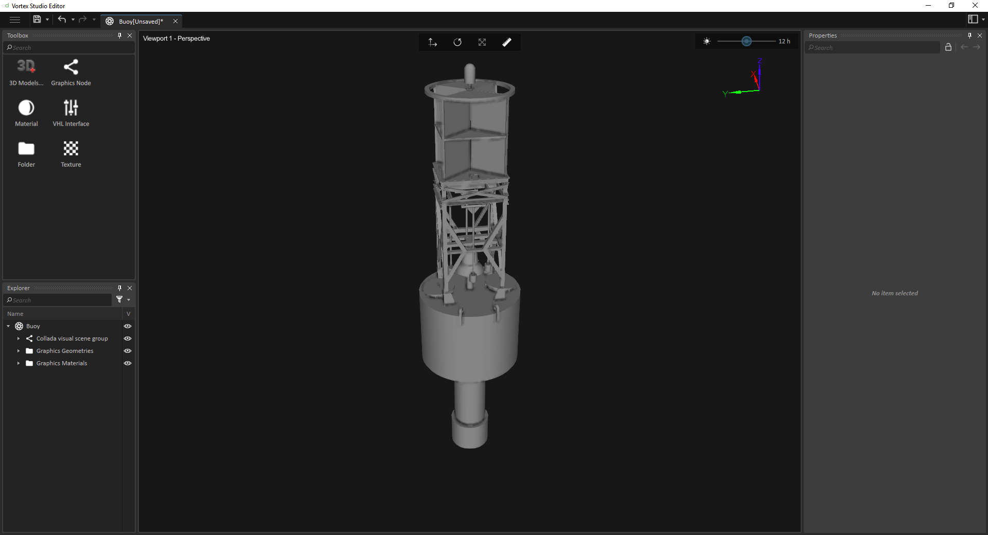
5. In the Explorer panel, you will find the 3D model within a Graphics Gallery that can be opened via the small triangle on the left. Doing so reveals these components:
   • Graphics Nodes: Each node contains a number of inputs and outputs, including visibility, transforms, etc. A node can have a graphics geometry and a graphics material, or neither.
   • Graphics Geometries: This folder contains the 3D meshes of the model.
   • Graphics Materials: This folder contains the graphics materials of the model.
6. Save the Graphics Gallery file by clicking the Save icon.

Clean Up Graphics Node Hierarchies

In this step, we will inspect the graphics nodes' hierarchy to ensure we only keep the nodes we need for building the simulation.

1. Right-click on a node in the Explorer panel to expand or contract the graphics nodes' hierarchy with the various Expand/Expand All/Collapse commands.
2. By right-clicking on a node (in the Explorer or viewport), use the Hide/Show commands to examine the model. Eliminate parts that are not useful (cables, piping, small bolts, etc.) or that will be hidden (internal parts).
3. Right-click on the Graphics Gallery in the Explorer panel and use Remove Orphans to eliminate leftovers (meshes, materials, and textures). Look over the list and press Enter to confirm.
4. See if any node is missing both graphics geometry and graphics material. They can often be eliminated, unless they are needed to apply a specific transform. If you need to delete a node:
   
   • Make sure the transform is preserved by its children (use the Move tool to display it, then right-click and select Bake Graphics Node on the child node).
   • Make sure to move out any child node from underneath its parent (otherwise, they will be deleted, too) by dragging it to its new location. Connections are automatically made.
   • Delete the empty node. 
5. Use Remove Orphans to eliminate leftovers.
6. Use the Hide/Show commands to examine the model. If nodes can be merged into one (e.g., bolts on a wheel), select the nodes with Ctrl + left mouse button.

7. Right-click and select Merge Graphics Nodes.
   

   Nodes can only be merged if they have the same graphics material.

8. Rename the new merged part for clarity.
9. Use Remove Orphans to eliminate leftovers.

Import Textures

1. From the Toolbox, double-click Texture.
2. From the Demo Scenes folder mentioned above (default location is C:\CM Labs\Vortex Studio Content <version>\Demo Scenes\Equipment\Buoy\Graphic\Buoy.dae), locate the image files using the browser. Load these textures.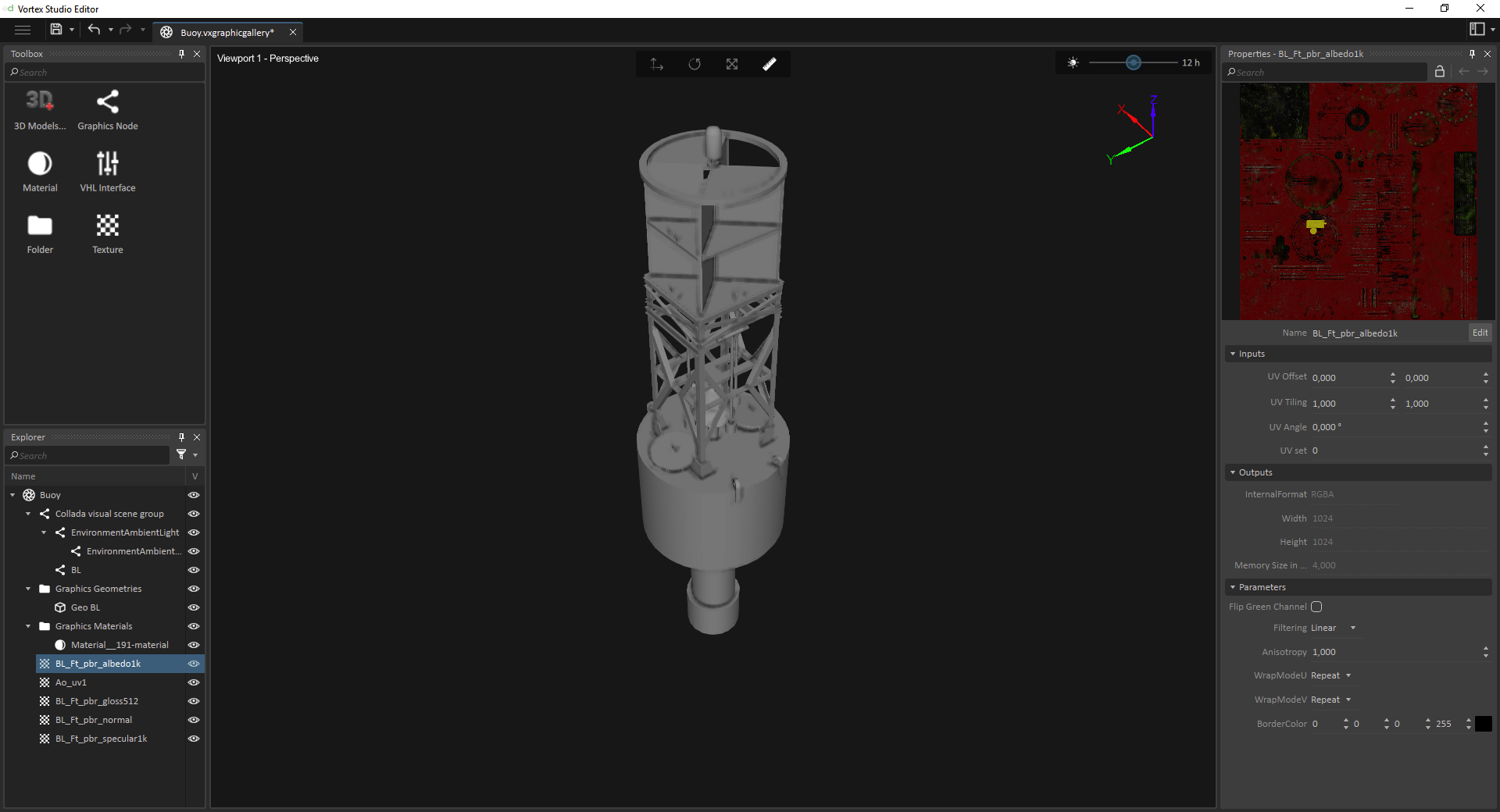
   
3. From the Toolbox, double-click Material. In the Explorer, select the new graphics material.
4. In the Properties panel, open the desired channel with the small triangle besides its name.
5. Add a layer with the + button, then match the loaded textures with their proper texture field by clicking on the ... button. A dialog box appears. The textures and their fields are:
   • Occlusion: Ao_uv1
   • Albedo: BL_Ft_pbr_albedo1k
   • Specular: BL_Ft_pbr_specular1k
   • Gloss: BL_Ft_pbr_gloss512
   • Normal: BL_Ft_pbr_normal
6. Locate the desired texture in the Explorer panel and click on it. Click check mark to confirm.
7. Repeat to link the other textures.

Check Textures and Adapt UV

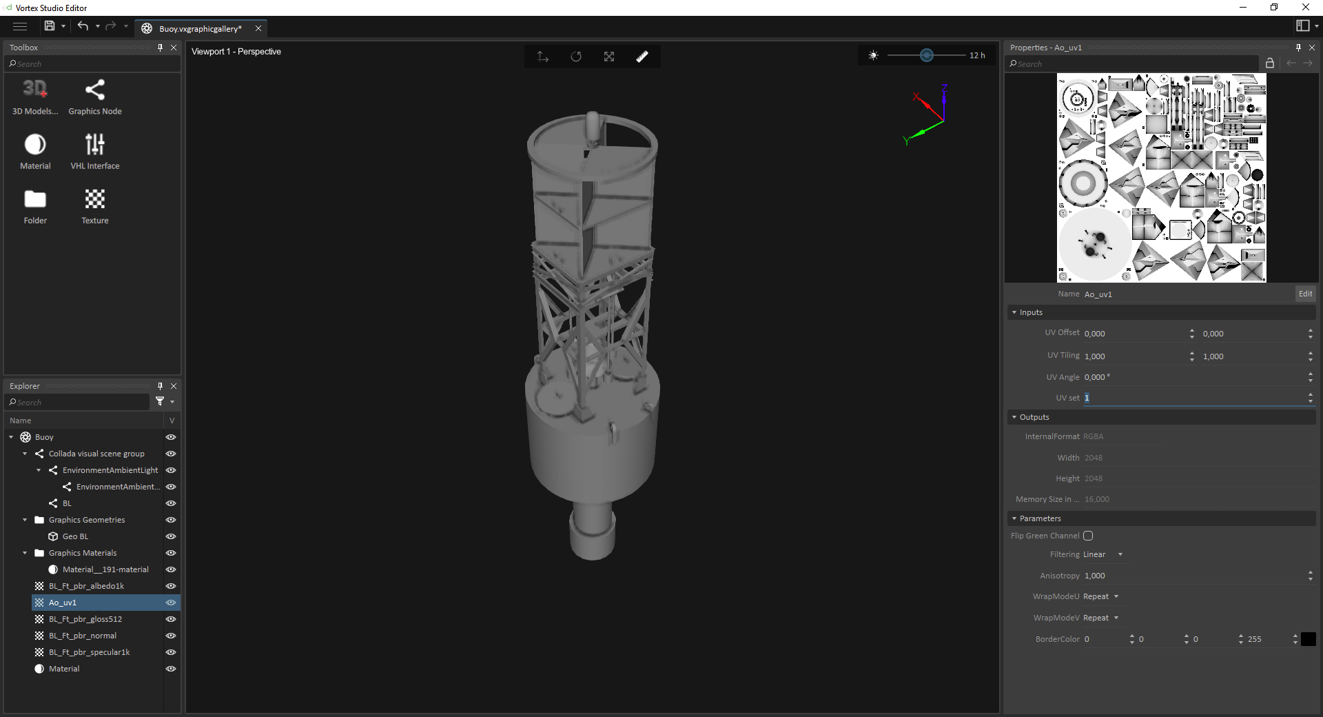
In this step, we will make sure the textures are properly placed and set to the right UV. For the buoy model, we need the ambient occlusion texture to be on its own UV set.

1. In the Explorer panel, locate the ambient occlusion texture (Ao_uv1).
2. In the Inputs section, change the UV Set to 1.
   

Check Model with Environment

In this step, we will activate the daylight feature and see how our model will appear in the simulation.

1. Select the BL node in the Explorer panel.
2. In its Properties panel, click "..." in the Graphics Material field.
3. In the resulting panel, select the new material you created. Click the check mark to confirm. The material is now applied to the model.
   
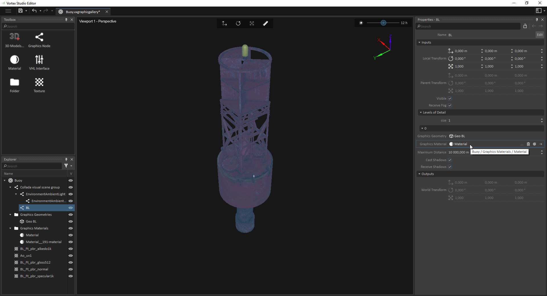
4. Click the Daylight button at the top-right of the 3D View. Use the associated slider to change the time of day.
5. Go back to each graphics material and change the values to adjust how the object responds to light.
6. In the Inputs section, select Environment Reflection. You can deactivate this feature if it affects the frame rate too much.
   

Clean Up the Graphics Gallery

In this step, we will clean-up our file names and structure to give more order to the model; this will make it easier to read by other users.

1. If it has not already been done by the 3D artist, the textures should be renamed for clarity according to a pre-set nomenclature.

   We suggest the following format:
   <name>_<texture use>_<resolution> (for example, BL_Ft_pbr_albedo_1k).

2. Make sure the name of each material accurately reflects its use.

   • Add the _mat suffix to make its nature obvious to other users.

3. Make sure the name of each geometry accurately reflects its use.
   • Add the _geo suffix to make its nature obvious to other users.
4. Every mesh and material should be located in the folder for that type. Drag any that aren't into the correct folder.

End Result

All textures and UVs are combined. We see that the contour is a texture that distorts the volume (normal map) and the ambient occlusion on a different UV set creates the suggestion of volume.

Click here to return to the main Tutorial Directory.