Constraint Types
- DEVOPS
This section lists the types of constraints that are available in Vortex®.
Angular 1 Position 3
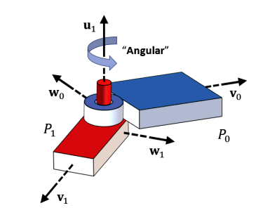
The "Angular 1 Position 3" is a general purpose two-part constraint, which is similar in nature to a Hinge or a Cylindrical but with additional positional control. It allows control of the parts' relative rotation around the first part's primary attachment axis and the relative position along the first part's primary, secondary and tertiary attachment axes. As such, it offers a total of four controllable coordinates. The coordinates are labeled Angular, Linear 0, Linear 1 and Linear 2.
The two remaining coordinates (relative orientation about secondary and tertiary axes) are not controllable. They appear in the Other Axes tab and can optionally be relaxed.
All controllable coordinates (linear and angular) are computed with respect to the axes specified in the first part attachment (see Attachments tab). A positive coordinate value represents a motion of the first part relative to the second part in the direction of the respective axis for a linear coordinate, or around this axis for an angular coordinate (respecting the right-hand rule for rotations).
The rotation induced by the angular coordinate (Angular) occurs around the center of the second part attachment.
Controllable Coordinates
| Name | Type | Effect |
|---|---|---|
| Angular | angular | Angular rotation about primary axis of first attachment. Point of rotation corresponds to second attachment position. |
| Linear0 | linear | Linear displacement along primary axis of first attachment. |
| Linear1 | linear | Linear displacement along secondary axis of first attachment. |
| Linear2 | linear | Linear displacement along tertiary axis of first attachment. |
Angular 2 Position 3
The "Angular 2 Position 3" is a general purpose two-part constraint, which is similar in nature to a "Universal" but offers additional positional control. It allows control of the parts' relative rotation around the first part's primary attachment axis and the second part's secondary attachment axis. It also gives control over the part's relative position along the first part's primary, secondary and tertiary attachment axes. As such, it offers a total of five controllable coordinates. The respective coordinates are labeled Angular 0, Angular 1, Linear 0, Linear 1 and Linear 2.
The remaining coordinate, relative orientation about the third attachment axis, is not controllable and appears in the Other Axes tab. It can optionally be relaxed.
The three positional (or linear) coordinates (Linear 0, Linear 1 and Linear 2) are computed with respect to the axes specified in the first part attachment (see Attachments tab). The two rotational (or angular) coordinates, Angular 0 and Angular 1, are computed with respect to the primary axis in the first part attachment and the secondary axis in the second part attachment, respectively.
A positive coordinate value represents a motion of the first part relative to the second part in the direction of an axis for a linear coordinate, or around an axis for an angular coordinate (respecting the right-hand rule for rotations). The rotations induced by the angular coordinates occur around the center of the second part attachment.
Controllable Coordinates
| Name | Type | Effect |
|---|---|---|
| Angular0 | angular | Angular rotation about primary axis of first attachment. Point of rotation corresponds to second attachment position. |
| Angular1 | angular | Angular rotation about secondary axis of second attachment. Point of rotation corresponds to second attachment position. |
| Linear0 | linear | Linear displacement along primary axis of first attachment. |
| Linear1 | linear | Linear displacement along secondary axis of first attachment. |
| Linear2 | linear | Linear displacement along tertiary axis of first attachment. |
Angular 3
The "Angular 3" is a general purpose two-part constraint that can be used to keep the relative orientation between two parts. It does not constrain either parts' position.
This constraint has three relaxable equations that appear in the Constraint Equations tab.
These equations are:
- Primary Axis Orientation
- Secondary Axis Orientation
- Third Axis Orientation
Controllable Coordinates: None
Ball and Socket
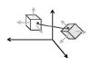
| A Ball and Socket is a two-part constraint which forces a point relative to one part to be at the same location as that of a point relative to the other part, removing three linear degrees of freedom between the two parts. As an example, in the provided diagram, the center of the sphere on one part always coincides with the center of the socket on the other part. The two coinciding points are defined in local space of the parts and can be specified in the first and second part attachments (see Attachments tab). This ideal joint allows all rotations about the common point and is also commonly referred to as spherical, or ball joint. The Ball and Socket has no controllable coordinates. However, the three linear coordinates which are constrained by the joint appear in the Other Axes tab and can optionally be relaxed.
|
Car Wheel
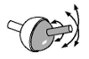
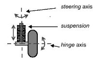
| The car wheel joint models the behavior of a car wheel, with steering and suspension. It is like a combination of two hinge joints (one for the steering and one for wheel rotation) along with a prismatic joint for the suspension. The first part is the chassis and the second part is the wheel. The connection point for the wheel part is its center of mass. The default steering axis is the Z-axis of the first part, and the default hinge axis is the Y-axis of the second part. Think of this constraint as having two main components: the steering column and driving axle, or steering and hinge components. The steering column is attached at point The axle can be made to rotate about the steering column in a plane perpendicular to it. This angle is controlled with either a position control or a limited-force, constant-velocity motor: for example, a motor which applies torque up to the specified maximum in order to achieve the specified velocity. The motion of the wheel about the axle is either free or controlled with another limited-force, constant-velocity motor. |
Cone
The Cone constraint is a specialized two-part constraint that limits the relative orientation between the two parts. It will prevent the angle between the primary axes of the first and second part attachments to exceed the specified Cone constraint angle. Note that the position of the part attachments is not relevant for the constraint's behavior and can be disregarded.
This constraint can be effectively combined with a Ball and Socket constraint which itself does not limit the relative orientation of the constrained parts.
Controllable Coordinates: None
Contact Gear
Contact Gear is a position-based constraint simulating the contact between the teeth of two gears.
The constraint takes two parts whose radii are provided as well as a backlash distance. Radius = 0 may be used to simulate a linear gear. In this case, the primary axis of the part is along the gear; otherwise, for circular gear, the primary axis is the rotation axis.
The constraint adds no force if the distance between the parts exceeds the sum of the radius (gears are disengaged).
The steps to follow for setting up this constraint are:
- Set the gear parts, axes and radii.
- Set the gear offset position so that one gear's teeth are positioned exactly between two of the other gear's teeth while simulating.
- Set the backlash distance so that the relative gears displacement is realistic.
- If the gear is allowed to jump teeth, set the gear max forces and teeth count for the circular gear so that accurate teeth thickness can be extracted.
Cylindrical
The cylindrical joint is a two-part constraint, which simulates a tubular block sliding on a cylindrical rod, thereby allowing both linear and angular movements between the attached parts. It acts like a prismatic and a hinge combined, thus removing four degrees of freedom between the two parts. The remaining two degrees of freedom, the Linear and Angular coordinates, can be controlled independently. This leaves four uncontrollable coordinates, two linear and two angular, which can optionally be relaxed via the Other Axes tab.
|
| Controllable coordinates Angular and Linear yielding rotation and displacement of the second part (P1) around the primary axis of the first part attachment (P0). Axes of i'th part attachment are indicated by the set of vectors {ui, vi, wi}. |

The cylindrical joint is not symmetric as its two part attachments have different geometric roles:
- The first part attachment represents the rod, which can be understood as a line in 3D space. The rod line is defined by the position and primary axis of the first attachment.
The linear and angular motion of the two attached parts, quantified by the two controllable coordinates of this joint, will occur along and around this line.
As the position and axes of the first attachment are specified relative to the first part, the rod is also fixed relative to the first part.
Consequently, if one of the two attached parts is static, it should be the first one, as this ensures that the rod line is fixed in world frame. - The second part attachment represents the block, which is is attached to the rod. The position of the second part attachment defines the location at which the block is attached to the rod, and slides along and around it.
Combined with relaxation of the two uncontrollable angular coordinates (see Other Axes tab), this point acts as a springy pivot.
Controllable Coordinates
| Name | Type | Effect |
|---|---|---|
| Angular | angular | Rotation of second part around the primary axis of the first part attachment. |
| Linear | linear | Displacement of second part along the primary axis of the first part attachment. |
Differential
The differential constraint is a velocity-based constraint that can take up to six parts and simulates a car's differential joint, the three first parts being the shaft and the two driven wheels, the three last parts being the reference for the three first ones respectively. The user can set the linear relationship between the angular velocities of the constrained parts. For instance, in a standard differential, the angular velocity of the drive shaft is equal to the average angular velocity of the output shafts.
The part's velocities are taken relative to the constraint attachment's primary axis relative to its reference part. In the case of a car's differential, as the wheels attached to the differential may be steered, the relative position of the wheels relative to their reference part, the chassis, will change. By default, the differential will recompute the reference part's attachment axis automatically so that the steered wheels won't cause problem.
Distance Joint
The distance joint is a position-based, two-part constraint that constrains the parts' attachment points to be within a given distance.
Controllable Coordinates: None
Double Hinge
The double hinge is like an assembly consisting of a hinge attachment fixed on one part, a distance constraint to a second part, and a hinge fixed on the second part. This can be used to simulate a torsion bar rod arm and wheel assembly on a tracked vehicle, for instance. The user controls the suspension of the torsion bar, the stiffness of the road arm, as well as the drive or brake on the rolling wheel.
Double Winch
This is a two-part constraint simulating the dynamics between two pulleys.
Given two pulleys of radius r0 and r1, this constraint computes the two line attachment positions and adds a distance constraint along this position, resulting in rotation only around the part attachment primary axis at the part attachment position.
As the line attachment may be going above or below the pulley, the secondary axis should indicate which side of the pulley to choose.
The distance constraint rest length corresponds to the initial distance between the line attachment and is updated according to the pulley's rotation as well as pulley's rotation around each other. Slack may accumulate.
If a pulley's radius is set to 0, the line attachment is identical to the part attachment. If the two radii are 0, then the constraint acts as a distance constraint.
The rotational axes of the two pulleys don't have to be parallel but they cannot be on the same line (as in the real world). If the line is pulled along the pulley's rotational axis, the line length will increase as if it is unrolling from the pulley.
Gear Ratio
The gear ratio constraint is a velocity-based constraint that constrains the velocity of a body relative to its primary attachment axis to the velocity of another body relative to its primary attachment axis. The gear supports up to four bodies where the third and the fourth bodies would be used as reference frame for the first and the second bodies respectively. This means that the gear will only act on the two first bodies' velocity relative to their reference bodies' velocity.
The part's velocities are taken relative to the constraint attachment's primary axis relative to its reference part. Normally the offset transform between a part and its reference part should be fixed.
Hinge
| The Hinge is a two-part constraint, which allows control of the parts' relative rotation around the second part's primary attachment axis (the hinge axis). The corresponding controllable angular coordinate is called "Angular". The remaining five coordinates appear in the Other Axes tab and can optionally be relaxed. The Hinge constraint can be used to attach a gate to a gatepost, a lever to its fulcrum, or a rotating part such as a wheel to a chassis, a propeller shaft to a ship, or a turret to a chassis. It removes five degrees of freedom between the two parts, and is therefore more computationally costly than, for example, a Ball and Socket constraint which removes three. A positive coordinate value of the Angular coordinate corresponds to a rotation of the first part relative to the second part around the hinge axis, respecting the right-hand rule for rotations. A rotation induced by the coordinate occurs around the center of the second part attachment. | ||||||
| Controllable coordinate Angular yielding a rotation of the first part (P0) around the primary axis of the second part attachment (P1). Axes of i'th part attachment are indicated by the set of vectors {ui,vi,wi}. | Controllable Coordinates
|
Homokinetic
A Homokinetic joint is similar to the universal joint, but exhibits no gimbal lock or rotational velocity variations. It constrains the rotation of the first part around its primary axis to the rotation of the second part around its primary axis and it also maintains relative positional constraint.
Linear 1
This constraint can be used to confine the linear motion of one part to a plane determined in the reference frame of a second part. A point fixed in the reference frame of the part 1 is constrained to a plane fixed in the reference frame of the part 2 or the global inertial frame. The point fixed in the reference frame of the first part is determined by the offset of part 1. The plane is determined by the primary axis of part 2, and is given by the plane normal to the primary axis. A position on this plane is determined by the relative offset of part 2. There are no controllable coordinates, but the single constraint can be optionally relaxed in the 'constraint equations' tab.
Linear 2
This constraint can be used to confine the linear motion of one part to a single axis determined in the reference frame of a second part. For this joint, a point fixed in the reference frame of part 1 is constrained to move along a line fixed in reference frame of part 2. The point on the first part is determined by the offset of the first part, for convenience, the origin of that line is called the joint position, and is determined by the relative offset of part 2, and the direction vector is called the joint axis and is determined by the primary axis of part 2. There are no controllable coordinates, but the two constraints can be optionally relaxed in the 'constraint equations' tab.
Linear 3
The geometry of this joint is such that during the simulation, a point fixed on part 1 will be on a line fixed in the reference frame of part 2. The line is defined by the offset and primary axis of the part 2 attachment. In addition, a direction vector fixed in the frame of part 2, and defined by the primary axis of the part 2 attachment, is fixed to be perpendicular to the axis of the line. There are no controllable coordinates, but the three constraints can be optionally relaxed in the 'constraint equations' tab.
Motor
The Motor constraint is a simple single coordinate constraint between two parts. It is similar to a Hinge or Prismatic constraint but only with the one controllable coordinate and no other restrictions which would remove degrees of freedom between the constrained parts. It can be used to actuate a part relative to another one, either leading to a linear displacement along the primary axis of the first attachment, or an angular rotation about the same axis, depending on the chosen constraint mode. The constraint mode of the Motor is angular by default but can be switched to linear by setting the Angular Motor input to false.
Controllable Coordinates
| Name | Type | Effect |
|---|---|---|
| Coordinate | linear or angular | If in angular mode, the constraint induces a rotation of the first part relative to the second part about the primary axis of the first part's attachment. If in linear mode (i.e., not in angular mode), the constraint induces a translation of the first part relative to the second part along the primary axis of the first part's attachment. |
Prismatic
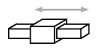
| The prismatic joint is imagined as a bar with a block that slides along it without rotating. The name prismatic refers to the imagined shape of the bar whose non-circular cross-section restricts rotation by keying into the matching hole in the block. A prismatic joint leaves a single, linear, degree of freedom (DoF) which can be controlled by a displacement coordinate. It constrains the two remaining linear DoFs and all three angular DoFs, as it acts to maintain the relative orientation of the parts. The prismatic joint is not symmetric as its two attachments have different geometric roles:
|
RPRO (Relative Position Relative Orientation)
 Relative Position Relative Orientation | RPRO, which stands for Relative Position Relative Orientation, is a robust quaternion-based multi-purpose constraint used for controlling the relative transform between two VxParts . A relative-position, relative-orientation joint can be used to join two simulated objects with a relative distance between them, as well as with a specified relative orientation. Parts joined by a relative-position, relative-orientation constraint that has not been relaxed have no freedom to move with respect to each other. In other words, the joint removes all six degrees of freedom from the attached parts. However, the relative orientation can be animated by supplying a sequence of relative quaternions and relative angular velocities. You can set one of the joint attachments to a specific location of a part and specify the relative orientation of that attachment with respect to the part's reference frame. An actual angular movement between the two bodies is done by updating the orientation between the two bodies using The relative transform between the two parts can be computed as follows. If A0 and A1 are the matrices corresponding to the attachments of part 0 and part 1 respectively, with columns formed by the primary, secondary and orthogonal axes, and if R0 and R1 are the part transform rotations, then the relative orientation between the two part coordinate systems is: R = R1 inv(A1) R0 A0. If you are changing the relative orientation dynamically, you must compute an angular velocity to help the constraint stabilize to the new value more quickly. |
Screw Joint
The Screw Joint constraint is a velocity-based constraint that constrains the angular velocity of a body along an axis to the linear velocity of another body around another axis. The screw joint supports up to 4 bodies where the third and the fourth bodies would be used as reference frame for the first and the second bodies respectively. This means that the screw joint will only act on the two first bodies' velocity relative to their reference bodies' velocity.
As this is strictly a velocity constraint, in general, the rotative part and the translative part constrained by other constraint.
Spring
The Spring is a two-part constraint which creates the dynamics of a damped harmonic oscillator (or spring-damping system) acting between the two parts. The spring-damper is attached between the positions specified in the two part attachments. The axes of the attachments are not relevant and do not influence the constraint behavior. This constraint has a single controllable coordinate, the Distance coordinate, which is computed as the current distance between the two attachments. The constraint force is always applied along the normalized vector passing through the two attachment positions (referred to as spring axis). For correct functioning, the Spring requires specification of the natural spring length (see Natural Length input), the distance between the two part attachments at which no elastic force is applied. If the relative velocity between the two parts is non-zero along the spring axis, a viscous damping force will be applied.
Specifically, the viscoelastic force F applied by the Spring constraint can be written as:
![]()
with natural spring length l, stiffness coefficient k, distance between the attachment points d, viscous damping coefficient c and the relative velocity between the two parts along the spring axis vr.
The Spring constraint tends to restore itself to its resting or natural length (the length at which no spring force is generated) by opposing any stretching or compression. Note that it is not recommended to set a natural length of approximately zero, as at zero distance between the attachment positions the spring axis can no longer be computed, and the behavior of the constraint is undefined.
The control mode of the Distance coordinate is always considered as "Locked". The modes "Free" and "Motorized" are not supported. The lock's Position input is equivalent to the Natural Length input and can be used to alter the rest length of the spring dynamically while simulating. Alternatively, a lock velocity can be specified which will update the lock position accordingly over time. It is advised not to shrink the natural length of the spring to zero as instabilities around this point are likely to arise.
Controllable Coordinates
| Name | Type | Effect |
|---|---|---|
| Distance | distance | Viscoelastic constraint force applied along spring axis (normalized vector between the two attachment positions). Coordinate control type can not be Motorized or Free. Only Locked mode is supported. |
Sum Distance
Sum Distance is a two-to-six parts velocity-based constraint that maintains the sum of the attachment distance to a constant value. The first and last part are rigidly connected while all parts in between are allowed to slide on the line as a pearl on a string.
For the moment, a given part can only appear once in the part list. With only two parts, the constraint acts as a velocity-based distance constraint. When computing the segment count, the count will stop when encountering one of the following:
- If two consecutive non-dynamics parts are encountered.
- If GetLineCount(segmentIndex) == 0
- If max part count was reached
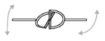
Universal
| In the universal joint two axes, one fixed in each of the two constrained bodies, are forced to have one point in common and to be perpendicular at all times. This is a lot like the ball-and-socket joint, except the ball is not allowed to twist in its socket. A universal joint removes four degrees of freedom from the attached bodies: it fixes their relative positions and also prevents them from twisting about a third axis, perpendicular to the two given axes. This joint can also be pictured as a joystick mechanism in which two hinges, with perpendicular axes, are joined one on top of the other, allowing an attached stick to move first in the x-direction then in the y-direction. This mechanism is also known as a gimbal, and suffers from the phenomenon of gimbal lock. Gimbal lock relates to the common use of the universal joint in transmitting torque from one body to another around a small bend. The transmission becomes increasingly unsmooth as the angle of bend approaches ninety degrees, and finally cannot transmit torque at all. |
Wheel
The Wheel constraint has four controlled coordinates: one for vertical; one for lateral; one for steering; and one for the wheel rotation along its axis. Each coordinate can be locked, motorized or limited. The longitudinal, lateral, yaw, roll and pitch displacements of the wheel can be constrained as functions of vertical displacement of the wheel described by tables. Using this constraint to attach a wheel to a chassis allows the user to simulate numerous types of chassis-wheel constraints.
Winch
The Winch is a useful four-part constraint that simulates the winch-pulley-hook-winchReference apparatus.
The constraint's part0 is the driving part whose movement, relative to part4, will be used, via a given ratio, to update the desired distance between part1 and part2 attachment positions.