Adaptive Cables
- DEVOPS
Cables in Vortex® are represented as a sequence of parts and constraints (or joints). The joints are configured such that, in sequence, they behave like a compliant cable with certain user-provided material properties. For more information on how to choose cable material properties, please refer to Cable Systems. Long cables can, depending on the selected preferred cable section length, have a very large number of joints (i.e., bending points), which makes their simulation computationally challenging. In order to maintain a minimally required simulation speed, as needed in real-time applications, Vortex provides an adaptive cable simulation scheme, which allows trading physical accuracy for simulation speed, while maintaining high fidelity cable dynamics.
In the adaptive cable scheme, only the cable joints which are required to accurately represent the cable's motion are simulated. Other joints are deactivated, hence greatly reducing the computational cost of this method. Based on the simulation type, this can yield impressive speed gains over fully simulated cables of the same length and with the same number of joints. In particular for subsea simulation scenarios (where due to fluid interaction forces, the cable dynamics are in general rather slow), the adaptive cable method can be successfully employed to improve simulation performance when it comes to modeling long tether cables.
|

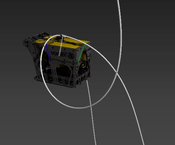
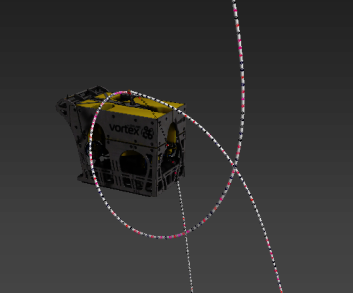
Long subsea tether cable with more than 1000 joints, simulated with adaptive cable technology.
As opposed to classical Level-of-Detail simulation approaches, the adaptive cable method does not change the cable's geometry by adding or removing cable elements. Instead, the cable's shape is maintained by selectively activating or deactivating cable joints according to the cable motion characteristics. This makes stable and robust collision behavior possible.
Deformations in the cable, which lead to joint activation, are detected through a joint motion estimation procedure which uses parallel processing of small-scale sub-simulations of currently deactivated cable portions to approximate the cable's dynamics, thereby leveraging Vortex's multi-threaded solver technology. As a consequence system resources can be effectively allocated to deforming cable regions while keeping the computation time at a minimum.
|
|
Setting Up Adaptive Cables
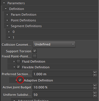
In order to use the adaptive cable feature for a cable segment, you must first enable it in your Dynamics Generic Cable Properties panel, as seen below.
Tuning Cable Simulation Fidelity
Once the adaptivity is enabled, joints will automatically deactivate if possible, thus speeding up the simulation. The physical accuracy of the cable simulation will be reduced while this feature is enabled; however, the loss is kept at a minimum through the adaptive joint activation.
A set of parameters provides the means to fine tune the balance between physical correctness and simulation speed. There are two types of parameters:
- Basic Parameters: Provide overall control over the balance between accuracy and speed in the cable simulation.
- Advanced Parameters: Provide finer control over the cable simulation (used only in rare cases).
Basic Parameters
| Name | Default Value | Description |
|---|---|---|
| Active Joint Budget | 10% | Defines the number of joints which can be activated as a percentage of the total number of joints in the cable. Activated joints are allocated to deforming cable regions, enabling cable deformation locally in the cable where needed. All other joints will remain inactive, thus reducing the computational time required for the cable simulation. Deforming regions are determined through a motion estimation procedure, in which, for each joint a sum of the joint's motion metrics (linear/angular joint acceleration/velocity) weighted by their respective coefficients (linear/angular joint acceleration/velocity coefficient) is computed. The obtained value defines a joint's relevance for the cable dynamics. The joints with the highest motion metric values are then activated until the entire Active Joint Budget is spent, or no more relevant joints are available (see table of joint coefficients below). The Active Joint Budget is given as percentage of the current number of joints in the cable. If the Active Joint Budget is set to 0%, the adaptive cable becomes a uniformly discretized cable (see Uniform Subdivisions). The higher this number, the more accurate the cable simulation becomes, but the more time is spent on cable simulation. |
| Uniform Subdivisions | 50 | Number of uniformly distributed active joints in the cable. This number provides the minimum number of active joints in the cable at any time, except if the cable has fewer joints. In addition to these active joints, the Active Joint Budget is used to activate joints in regions where cable deformation occurs. |
Advanced Parameters
| Name | Default Value | Description |
|---|---|---|
| Maximum Active Joint Count | 400 | This number is used to limit the number of active joints in the Active Joint Budget. The cable will never have more active joints than the Maximum Active Joint Count, except if the number of Uniform Subdivisions is higher. This parameter can be used to limit the computational complexity in the simulation in cases where a cable becomes very long, and the Active Joint Budget would become too high to maintain real-time simulation rates. |
| Maximum Motion Sample Count | 4 | Maximum number of samples used in cable motion estimation. Joint motion in inactivated cable regions is estimated in order to detect cable deformations which should occur at these locations. This parameter defines the number of samples taken for this purpose in any cable region with inactive joints. See also Active Joint Budget. A high value will lead to a more accurate cable motion estimation but will increase computation time. |
| First Boundary Active Joints | 2 | The number of joints in the flexible cable that won't be adaptive at the first extremity. |
| Last Boundary Active Joints | 2 | The number of joints in the flexible cable that won't be adaptive at the last extremity. |
Fine-Tuning
The following parameters are used to fine-tune the motion estimation algorithm.
Motion in the cable is computed on a per joint basis. Joints which have a high motion metric are candidates for joint activation. The motion metric of a joint is computed as a weighted sum of the following kinematic quantities:
- Angular joint velocity
- Linear joint velocity
- Angular joint acceleration
- Linear joint acceleration
A weight applied to each of the above kinematic quantities allows tuning the effect they have on the motion metric and thus on the probability that a joint will be activated in a certain situation. These weights are:
- Angular joint velocity coefficient
- Linear joint velocity coefficient
- Angular joint acceleration coefficient
- Linear joint acceleration coefficient
These parameters are used to calculate a motion metric for a joint. The higher this value, the more likely it is that the joint will be activated.
The table summarizes the relevant parameters.
| Name | Default Value | Description |
|---|---|---|
| Linear Joint Acceleration Coefficient | 1.0 | Used as a weighting factor during joint motion estimation to determine if a cable joint is relevant for the cable dynamics. A higher value will give more priority to joints exhibiting a linear acceleration when deciding which joints to activate. |
| Linear Joint Velocity Coefficient | 10.0 | Used as a weighting factor during joint motion estimation to determine if a cable joint is relevant for the cable dynamics. A higher value will give more priority to joints exhibiting a linear velocity when deciding which joints to activate. |
| Angular Joint Acceleration Coefficient | 1.0 | Used as a weighting factor during joint motion estimation to determine if a cable joint is relevant for the cable dynamics. A higher value will give more priority to joints exhibiting an angular acceleration when deciding which joints to activate. |
| Angular Joint Velocity Coefficient | 10.0 | Used as a weighting factor during joint motion estimation to determine if a cable joint is relevant for the cable dynamics. A higher value will give more priority to joints exhibiting an angular velocity when deciding which joints to activate. |
Furthermore, in order to prevent activating joints which show close to no motion at all, motion thresholds can be defined for each kinematic quantity. If all kinematic quantities of a given joint fall below these thresholds, it will not be considered for activation. In periods of low overall cable motion, this prevents activating irrelevant joints in the cable and thus unnecessarily up computational resources.
The corresponding parameters are as follows.
| Name | Default Value | Description |
|---|---|---|
| Minimum Angular Joint Acceleration | 10.0 °/(m*s2) | Minimum angular acceleration of cable joints for motion estimation. Specified as angular acceleration per unit length. Used as a cut-off value during joint motion estimation to determine if a cable joint is relevant for the cable dynamics. If a given joint's angular acceleration falls below the provided value, it will not be activated during Active Joint Budget allocation. |
| Minimum Linear Joint Acceleration | 1.0 /s2 | Minimum linear acceleration of cable joints for motion estimation. Specified as linear acceleration per unit length. Used as a cut-off value during joint motion estimation to determine if a cable joint is relevant for the cable dynamics. If a given joint's linear acceleration falls below the provided value, it will not be activated during Active Joint Budget allocation. |
| Minimum Angular Joint Velocity | 1.0 °/(m*s) | Minimum angular velocity of cable joints for motion estimation. Specified as angular velocity per unit length. Used as a cut-off value during joint motion estimation to determine if a cable joint is relevant for the cable dynamics. If a given joint's angular velocity falls below the provided value, it will not be activated during Active Joint Budget allocation. |
| Minimum Linear Joint Velocity | 0.1 /s | Minimum linear velocity of cable joints for motion estimation. Specified as linear velocity per unit length. Used as a cut-off value during joint motion estimation to determine if a cable joint is relevant for the cable dynamics. If a given joint's linear velocity falls below the provided value, it will not be activated during Active Joint Budget allocation. |
Note that these threshold parameters are all specified in units per cable unit length, which makes them independent from the cable resolution (i.e., the number of joints in the cable).
To help understand this better, consider a simple cable with only a single joint. When the cable begins stretching with a certain velocity, the linear velocity of the joint will change. Let's assume that, after changing the cable resolution, the same cable now has two evenly spaced joints instead of one. If the entire cable is stretched as before, the stretching velocity will now be distributed over the two joints, reducing the joint velocities accordingly. This observation shows that a threshold on the stretching velocity per joint must be independent of the number of joints. Otherwise, the threshold would be surpassed for a cable with one resolution (e.g., one joint with high linear velocity) but not for another (e.g., two joints with lower linear velocity). This would drastically change the joint activation process and lead to unexpected differences in simulation.
Therefore, when a joint's velocity or acceleration is compared with the given threshold in an adaptive cable, the threshold is multiplied with the uniform spacing between the cable joints. This counteracts the effect the cable distribution has on the joint velocities and explains why the thresholds must be specified per unit length.