Tire Models Technical Notes
- DEVOPS
Tire Models Technical Notes
The tire models provided in the Vortex® toolkit are based on real scientific research. This page is meant to provide more technical background information than is found in the Adding Tire Models section.
Tire Normal Force
When the hard ground tire model is used, the stiffness at the contact patch is deduced from the tire pressure. Tire pressure can be set to infinity in cases where no compliance in the contact is desired.
When a soft ground tire model is used, the stiffness at the contact patch is computed based on the pressure-sinkage parameters described in Tire Models. The pressure at any point of the tire-soil interface is calculated based on the pressure-sinkage relationship. The normal force is obtained by integrating the pressure along the tire-soil interface. The contribution of shear stress is also considered in computing the normal force. The tire stiffness based on the tire pressure is combined to the stiffness from the soft ground model. This contribution vanishes if the tire pressure is set to infinity.
Hard Ground Tire Models
The following section describes the hard grounds tire models. Each model is used to compute the longitudinal and lateral friction force (the traction and the cornering, respectively), and the alignment moment (which is along the normal vector at the contact). The stiffness at the contact patch is computed based on the tire pressure, and the rolling resistance depends on the actual rolling resistance model in use.
Magic Formula (1997 and 2002 Pacejka models)
Note The following information relates only to the 1997 Magic Formula model. For the Pacejka Magic Formula 2002 model, make sure you are using the correct data before using it. The explanation for the 2002 model is beyond the scope of this documentation but is readily available online.
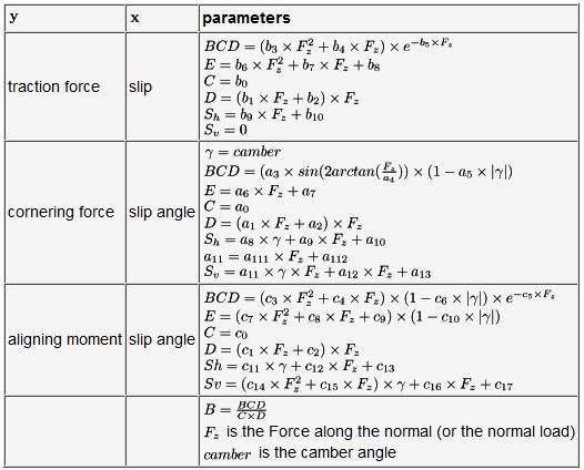
The Magic Formula Tire Model is based on the work by Pacejka et al 2805435586, 2805435586, 2805435586, 2805435586. It uses mathematical functions that relate the lateral force as a function of lateral slip, the longitudinal force as a function of longitudinal slip, and the aligning moment as a function of lateral slip.
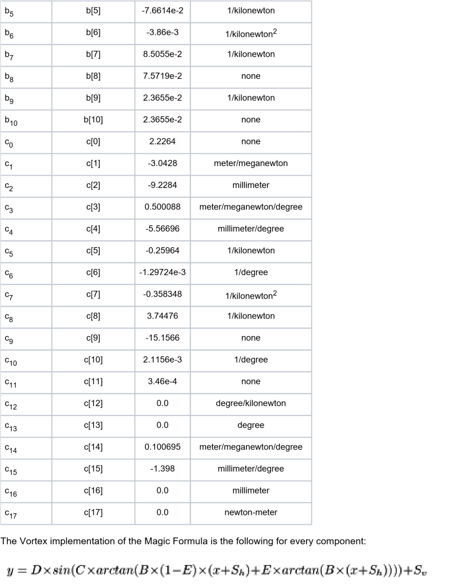
The following table shows the default values of the magic formula.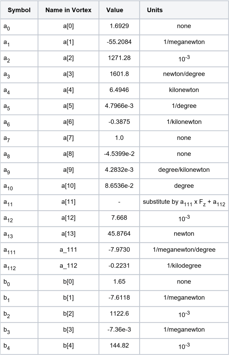
Composite Slip Tire Model
The Composite Slip Tire Model is based on the work by Szostak et al 2805435586 . This model produces tire forces taking into account the interaction of longitudinal and lateral forces from small through saturation. Tire longitudinal and lateral forces are computed from composite force which is a function of composite slip. The composite slip is computed from slip angle, longitudinal slip, normal load, tire patch length, friction coefficient, longitudinal and lateral stiffness coefficients, etc.
The next table shows the default value of the composite slip tire model.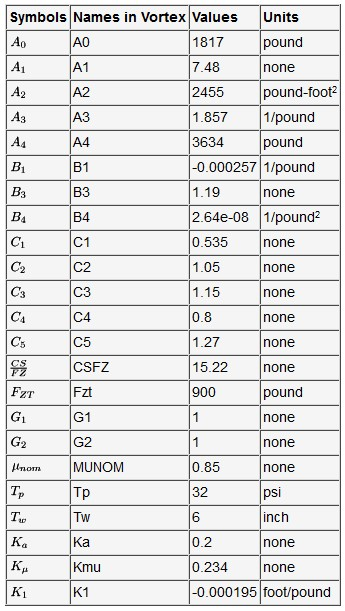
Example of values for three types of tire 2805435586 :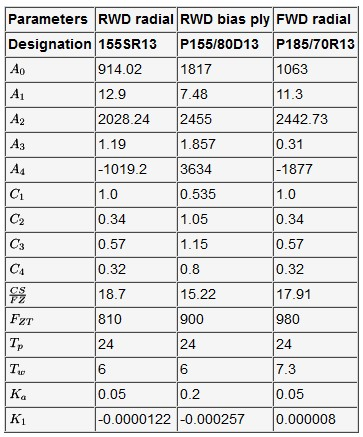
norm should be 0.85 for normal road conditions, 0.3 for wet road conditions, and 0.1 for icy road conditions.
Fiala Tire Model
The Fiala tire model is based on the work by Fiala 2805435586 . This model uses the parameters that are directly related to the physical properties of the tire to determine tire longitudinal forces, lateral forces, and aligning moments. Note that the carcass radius is used only in the case of the alignment moment.
According to that theory, in case where there is no lateral slip, the maximum traction force would be:![]()
where N is the load applied on the wheel.
The slip value where half of the maximum traction happens is called the critical slip and is represented by:![]()
A typical value for the critical slip is around 15%.
The following table shows the default values of the Fiala tire model in Vortex. They are based on a wheel load of 5000 newtons and critical slip of 15%.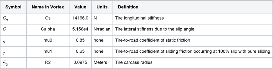
Coulomb Friction Model
The Coulomb friction model is not like the other hard ground tire models. It has been introduced in Vortex to give the possibility of using the classic friction models of Vortex in the same way as the other tire models (see VxMaterial for more details). Note that the Coulomb tire model has been stripped of a few properties that were not relevant for tire interaction with a hard ground. For instance:
Stiffness/compliance has been removed since tire pressure models it (note that the damping has been kept as a scaling factor on the critical damping).
Restitution has been removed since this feature is more likely to be used for pure elastic contact interaction.
Friction around the three axes have been removed: Around the primary axis of the contact, friction is not needed. Around the secondary axis of the contact, the rolling resistance model (if set) gives a more realistic result. Finally, around the normal axis, the friction is implicitly added by the lateral and the longitudinal friction of the two contacts at the tire patch.
The default value of the Coulomb tire models is as follow: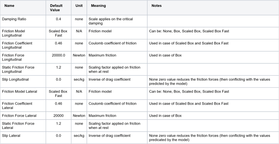
Soft Ground Tire Models
The Soft Ground Tire Model as implemented in Vortex is mainly based on the work by Bekker 2805435586, 2805435586, 2805435586 and Wong 2805435586, 2805435586 . The tire normal and shearing forces are computed by integrating normal pressure and shear stress over the entire tire-terrain contact area. In order to find normal stress distribution under the wheel, an appropriate pressure-sinkage relation should be used depending on the type of soil with which the wheel is interacting (in terramechanics literature, the pressure-sinkage relation is the relation between average pressure under a rigid plate versus the penetration depth). Then, we need a model to relate these pressure-sinkage relations to the pressure under the wheel. Various available models in the literature have been implemented in Vortex. In Vortex, the pressure-sinkage model refers to the combination of a particular pressure-sinkage relation and a model relating it to a rolling wheel. These include Bekker, Bekker-Wong, Reece, Muskeg, and Snow.
The shear stress-shear displacement relationship is characterized by the exponential shearing equation, the hump shearing equation, or the Wong shearing equation. This is detailed in section Shear Stress-Shear Strain Models.
Pressure-Sinkage Models
Bekker
The Bekker equation is the default pressure-sinkage equation for Soft Ground Tire Models in Vortex, which is used to represent the pressure-sinkage characteristics of homogeneous terrain, such as sand and clay. It is given by:![]()
where p is the pressure, b is the smaller dimension of the contact patch, z is the sinkage and n, kc, k are the pressure-sinkage parameters. In this model, the normal stress distribution under the wheel is obtained by the relation below:![]()
The following is a schematic of rigid wheel and soil contact.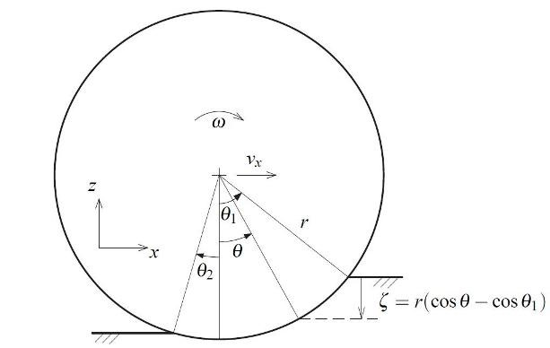
The exit angle θ2 is assumed to be zero in this model. The default values (corresponding to sandy loam) for Bekker parameters are shown in the table below.
Values for a sample of terrains are given in 2805435586 .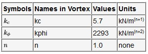
Bekker-Wong
An alternative way to represent normal stress distribution under a wheel is developed by Wong and Reece 2805435586. Contrary to the Bekker model, maximum normal stress distribution may not occur at the bottom-dead-centre of the wheel. They proposed the empirical relation below for estimating θm as the location of the point of the maximum radial stress:![]()
where a0 and a1 are dimensionless constants, θ1 defines the location of the point corresponding to the beginning of wheel-soil contact, and i is the wheel slip ratio defined by:![]()
Based on this model, normal stress distribution is obtained using the next relations:![]()
![]()
where θ2 is the exit angle. θ2 is assumed to be zero in this model.
The default values for Bekker-Wong parameters are shown in the table below.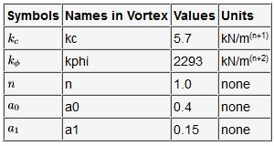
Reece
The pressure-sinkage relationship is characterized differently in the Reece model (compared to the Bekker's parameters):![]()
where c is soil cohesion, γs is weight density or specific weight of terrain, z is the wheel sinkage, and b is the wheel width or the smaller dimension of the contact patch. k'c and k'φ are the new pressure-sinkage parameters, which are dimension-less, and n is the pressure-sinkage exponent. In this model, θm is calculated similar to the Bekker-Wong model. Normal stress distribution under the wheel is then calculated using the relations below 2805435586:![]()
![]()
In this model, θ2 can be non-zero. Following an approach explained in 2805435586 , θ2 is calculated by the relation below:![]()
where λ is a dimensionless parameter that can have a value from 0 to 1. The default values for Reece parameters are shown in the table below.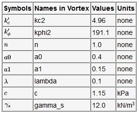
Muskeg
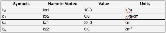
The Muskeg equation is used to represent the pressure-sinkage characteristics of various types of organic terrain (muskeg):![]()
where p is the pressure, z is the sinkage, kp is a stiffness parameter for the peat, mm is a strength parameter for the surface mat and Dh is a value (in meters) related to the contact area. Dh = 4 A/L where A and L are the area and the perimeter of the contact patch, respectively.
Normal stress distribution under the wheel is obtained using the following relation:![]()
The default values for Muskeg (corresponding to Muskeg type A) parameters are shown in the table below.
Values for a sample of terrains are given in 2805435586.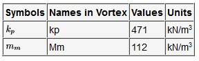
Snow
The Snow equation is used to represent the pressure-sinkage characteristics of snow on top of ice layers:![]()
where p is the pressure, z is the sinkage and D is the smaller dimension at the contact patch (in cm). Normal stress distribution under the wheel is obtained using the relation below:![]()
The default values for Snow parameters are shown in the table below, see 2805435586 .
Pressure-sinkage Multi-pass Models
Soft ground tire models can include the effect of soil hardening caused by wheels passing over an area multiple times. This is of primary importance for vehicles with multiple wheels or terrains that will be driven over multiple times, as each wheel changes the mechanical properties of the soil when it has passed over it.
By using this feature:
- Wheels can permanently deform the ground surface, leaving ruts.
- More accurate motion resistance is computed.
- More accurate prediction of traction force is computed.
To include this effect in the simulation, the ground surface must be modelled with a Deformable Terrain or an Earthwork Zone. Three pressure sinkage relations are supported: Bekker, Wong, and Reece. (Muskeg and Snow do not model mineral-based soils, therefore they are not supported). Each of these has a parameter named Enable Soil Hardening that must be set.
A description of the concepts can be found in Wong2805435586 2805435586, where a description of the effects of ground response to repetitive loading is given.
The next section gives an overview of the concept.
Response to Repetitive Loading
From experiments, it has been observed that when a small surface of ground is loaded for the first time, the pressure increases with the sinkage according to the pressure sinkage relations (gray line in the picture below). If the pressure is released (at penetration zu), the soil surface rises up to bu (because of its elasticity) then stops even if no load is applied anymore. The soil surface is then permanently deformed. This is called plastic deformation.
If a load is subsequently applied to the same area, the experimental observation shows that the pressure will increase approximately linearly with the sinkage (along the black line) until the sinkage reaches the point where the load was released the first time (zu). If the load is increased further, the pressure continues to increase following original pressure sinkage relation curve (gray). In the picture, the elastic range of z is labelled e.
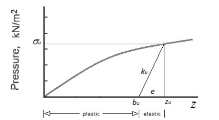
When the sinkage z is within the elastic range, the pressure takes the form:![]() where z is in [e]
where z is in [e]
ku represents the rate of increase of pressure in the elastic range.
Again, following references 2805435586 2805435586, it has been shown experimentally that the elastic stiffness ku in the elastic range depends on the level of sinkage in the following form:![]()
Where k0 and Au are parameters that can be determined from experimental data.
In cases where k0 and Au are not available, the following section suggests a procedure to choose these parameters. They control the size of the plastic and the elastic portions of the soil in case of repetitive loading.
Choosing k0 and Au
The parameters k0 and Au are used to determine the plasticity and elasticity of the soil. When those parameters are known from experimental results, it is suggested to use them. For cases where these parameters cannot be found, this section gives a procedure to determine approximate values for k0 and Au that will represent realistic soil behavior.
Choosing k0 and Au from Elasticity
The idea behind this procedure is to choose the amount of elasticity at two values of z in the pressure sinkage diagram. This is represented by penetrations z1 and z2 and the length of elasticity represented by e1and e2 in the next diagram.
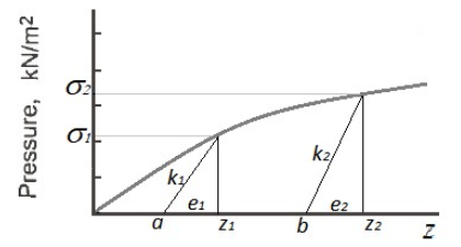
Following the repetitive loading principle, at penetration zi, the soil stiffness is given by:![]() (1)
(1)
where i is 1 or 2.
On the other hand, ki can be seen as the rate of change of pressure during a second pass:
![]() (2)
(2)
Where we have written keq as a constant for a given pressure sinkage relation:
![]()
Here, kc and kΦ are the pressure sinkage parameters and b is taken as the width of the wheel (using Bekker's representation in this example).
By choosing a length of elasticity at two different penetrations points, we can use (1) and (2) to form a system of two equations for the two unknowns ko and Au.![]()
![]()
By solving for k0 and Au, we find:![]()
![]()
Here, keq and n are from the current pressure sinkage relation, and z1, z2, e1 and e2 are user-desired penetration and elasticity lengths.
This technique to choose the parameters k0 and Au gives approximate values as it does not consider the actual shape of the wheel.
The procedure has been captured in the following Python script (using Bekker relation):
#wheel width
W = 0.205 # Wheel width in meters
assert (W>0), "invalid wheel width {}".format(W)

# pressure sinkage parameter (units depends on parametrization)
n = 0.97
Kc = 5.5
Kphi = 2293

assert(n>0), 'invalid exponent in pressure parameter {}'.format(n)

# desired penetration and elastic length at two points in meters
z1 = 0.02
e1 = 0.01
z2 = 0.04
e2 = 0.005

#validation:
assert(z1>0),'z1 must be strictly larger than 0 z1={}'.format(z1)
assert(e1>0.0), 'e1 must be strictly larger than 0 e1={}'.format(e1)
assert(z1<z2), 'z2 must be strictly larger than z1 z1={} z2={}'.format(z1,z2)
assert(e2>0),'e2 must be strictly larger than 0 e2={}'.format(e2)

Keq = ( Kc/W + Kphi ) # this example is for Bekker
C1 = Keq*(z1**n)
C2 = Keq*(z2**n)

# results
K0 = (C1*z2 / e1 - C2*z1/e2)/(z2-z1)
Au = (C2/e2 - C1/e1)/ (z2-z1)
print ( 'K0 = {} and Au = {} '.format( K0, Au) )
Shear Stress-Shear Strain Models
In soft ground tire models, the traction force is based on the shear stress-shear strain characteristics of the soil. Soft ground tire models implement three different soil shearing properties. In each of them, they give the ratio of shear force to the maximum shear force, smax, as a function of the shear displacement (noted j in future equations). The maximum shear force occurs at the point where the shear displacement produces a failure of the soil. This point is commonly characterized by the Mohr-Coulomb failure criterion given by:![]()
Exponential
The Exponential equation is the default shearing equation, which is used to represent the shear stress-displacement characteristics of loose sand, saturated clay or fresh, dry snow. This model was proposed by Janosi and Hanamoto2805435586.
In this case, the relative shear force is given by:![]()
The default values for Exponential Shearing parameters are shown in the table below.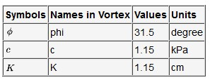
Hump
The Hump equation has a distinct "hump" of shear stress with a subsequent decrease to a value approaching zero. It has been used to represent the shearing characteristics of some types of muskeg mats.
In this case, the relative shear force is given by:![]()
The default values for Hump Shearing parameters are shown in the table below.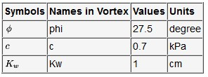
Wong
The Wong equation is similar to the Hump equation, but it allows a level of residual shear stress sr rather than dropping to zero after the hump. It is useful in representing the shearing characteristics of some types of snow and loam, usually in a compacted state.
In this case, the relative shear force is given by:
Where Kw is the shear displacement (in cm) where the maximum shear stress appears and Kr is the residual shear stress.
The default values for Wong Shearing parameters are shown in the table below.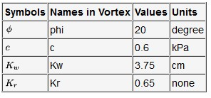
Lug
In Vortex soft ground tire models, the traction force is based on the shear stress-shear strain characteristics as explained in the previous section. Moreover, the traction force includes the effect of the lugs. Therefore, the traction force is the combination of the internal shearing model (at the carcass) and the external shearing model (at the surface of the lug). The effect of the two models is averaged in proportion of the lug-to-carcass ratio. The actual contribution from the carcass depends on the sinkage and the lug height. In case where the lug's height is zero, the two ratios are ignored, and 100% of the traction comes from the Internal Model.
The default values for lug parameters are shown in the table below.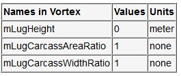
Lateral Force
The lateral force is modelled as an exponential function of slip angle integrated over the contact area between the tire and the terrain.
where cs is given by:![]()
In these equations, Fl is the lateral force, A is a user constant, W is the tire width, R is the wheel radius, sa is the slip angle (in radians), and p(θ) is the pressure under the tire. It depends on the actual normal stress distribution. Please, refer to the diagram in the 2805435586 model section above for notation. As this formulation gives no lateral force when lateral slip is zero (also called the slip angle), the model provides a way to set a minimum value for cs.
The default values for lateral force parameters are shown in the table below. Note that A=0 is enough to obtain no lateral force.
| Names | Values | Units |
|---|---|---|
| A | 1.5 | None |
| B | 0.2 | rad-1 |
| Min. Threshold Coeff | 0.0 | None |
Tire Pressure
Although the effect of the tire pressure is not included in any theoretical tire models, Vortex takes it into account in a few ways.
The tire pressure is used to compute the normal stiffness at the contact and this introduces some tire deflection.
In case of soft ground (2805435586 and 2805435586 only), it affects the sinkage, which has two consequences. First, it affects the compaction resistive force, and second, it affects the shear stress which in turn affects the traction force.
The deflection of the tire caused by the tire pressure also generates some rolling resistance torque. This is discussed below in 2805435586.
The tire pressure is given in pascals and the default value is 220627.2 Pa (which is equivalent to 32.0 Psi).
Rolling Resistance
The resistance in the tire-terrain interaction is composed of two parts in the tire model. One part, which is referred to as compaction resistance, is related to the compaction of the terrain, and it is computed and implemented in the soft ground tire model. This resistance is zero in the other tire models.
The other part of the resistance is referred to as rolling resistance; it is due to the deformation of tires, and it is computed and implemented in the tire model base on different models available. Note that soft ground tire models include resistive torque and force caused by the soil compaction and that the effects of the rolling resistance models are added to it.
The rolling resistance is computed based on the rolling resistance coefficient. The rolling resistance coefficient represents the ratio of the rolling resistance to the tire normal force. Depending on the type of rolling resistance model that is selected, it can be a function of only forward wheel speed or it can also depend on tire pressure and normal force. The rolling resistance induces a resistive torque of the form:![]()
Where cr is the coefficient of rolling resistance, R is the wheel radius and N is the normal force on the wheel; cr is unit less.
There are three different models:
2805435586 , 2805435586 and 2805435586 .
Rolling Resistance Speed Model
In this model, the coefficient is a function of the linear speed of the wheel.![]()
The default values for these coefficients are all zero.
Rolling Resistance Tire Pressure Model
In this model, the coefficient is a function of the linear speed of the wheel and the tire pressure.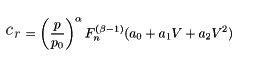
Where p is the current tire pressure, p0 is the nominal tire pressure, Fn is the load, alpha is the tire pressure exponent, and is the normal load exponent.
The default values for this coefficient model are: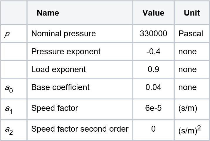
Rolling Resistance Table Model
In this model, the coefficient is given by a look-up table provided by the user as a CSV file containing two columns. In the first column, we must have linear speed of the wheel in meter per second (must appear in increasing order). The second column contains the rolling resistance coefficient.
The default table given in the resources folder is 2805435586:
| Speed (m/s) | Coefficient |
|---|---|
| 5.55 | 1.00 |
| 19.44 | 1.00 |
| 27.78 | 1.03 |
| 33.33 | 1.11 |
| 36.11 | 1.14 |
| 38.89 | 1.2 |
| 44.44 | 1.3 |
References
[1] H.B. Pacejka, ``The Tyre as a Vehicle Component", Proc. XXVI FISITA Congress, Prague, June 16-23, 1996 (CD-ROM).
[2] E. Bakker, L. Nyborg, and H.B. Pacejka, ``Tyre Modelling for Use in Vehicle Dynamics Studies," Society of Automotive Engineers, paper 870421, 1987.
[3] E. Bakker, H.B. Pacejka, and L. Lidner, ``A New Tire Model with an Application in Vehicle Dynamics Studies," Society of Automotive Engineers, paper 890087, 1989.
[4] H.B. Pacejka and I.J.M. Besselink, ``Magic Formula Tyre Model with Transient Properties," in F. Bohm and H.-P. Willumeit, Eds., Proc. 2nd Int. Colloquium on Tyre Models for Vehicle Dynamic Analysis, Berlin. Lisse, The Netherlands: Swets & Zeitlinger, 1997.
[5] G. Genta, Motor Vehicle Dynamics: Modeling and Simulation, World Scientific, Singapore, 2003
[6] H.T. Szostak, ``Analytical Modeling of Driver Response in Crash Avoidance Maneuvering Volume II: An Interactive Tire Model for Driver/Vehicle Simulation", National Highway Traffic Safety Administration Report DOT-HS-807-271, 1988
[7] E. Fiala, ``Seitenkrafte am rollenden Luftreifen," VDI-Zeitschrift 96, 973, 1954.
[8] J. Blundell, D. Harty, The Multibody Systems Approach to Vehicle Dynamics, Elsevier Butterworth-Heinemann, Burlington, MA, USA, 2004.
[9] M.G. Bekker, Theory of Land Locomotion, The University of Michigan Press, 1956.
[10] M.G. Bekker, Off-The-Road Locomotion, The University of Michigan Press, 1960.
[11] M.G. Bekker, Introduction to Terrain-Vehicle Systems, The University of Michigan Press, 1969.
[12] J.Y. Wong, Theory of Ground Vehicles, John Wiley, New York. 3rd Edition, 2001.
[13] J.Y. Wong, Terramechanics and Off-Road Vehicles, Elsevier Science Publishers, Amsterdam, the Netherlands, 1989.
[14] J.Y. Wong and A.R. Reece, ``Prediction of Rigid Wheel Performance Based on the Analysis of Soil-Wheel Stresses Part I: Performance of Driven Rigid Wheels," J. Terramechanics, 1967, vol. 4, 81-98.
[15] G. Ishigami, A. Miwa, K. Nagatani, and K. Yoshida, ``Terramechanics-based model for steering maneuver of planetary exploration rovers on loose soil," J. Field Robotics, 2007, vol. 24, 233-250.
[16] T.J. LaClair, The pneumatic tire: Chapter 12, Rolling resistance, U.S. Department of Transportation, National Highway Traffic Safety Administration, DOT HS 810 561, February 2006.
[17] Z. Janosi and B. Hanamoto, “The analytical determination of drawbar pull as a function of slip for tracked vehicles in deformable soils,” in Proceedings of the ISTVS 1st International Conference on Mechanics of Soil-Vehicle Systems, pp. 707–736, Edizioni Minerva Tecnica, Torino, Italy, 1961.2805435586
[18] The Pneumatic Tire, U.S. Department of transportation, National highway traffic safety administration DOT HS 810 561 (2006)