Dynamics Performance Analysis
- DEVOPS
This document contains information regarding the tools provided by Vortex® Studio to help find dynamics performance issues. Please refer to the Performance Analysis guide for an overview.
Finding Bottlenecks in the Physics Engine
If The Profiler tab in the Vortex Studio Player indicates excessive time consumption in the dynamics module (usually called DynamicsEngine in your application setup) you can modify your simulation content or tune simulation parameters to reduce the time spent.
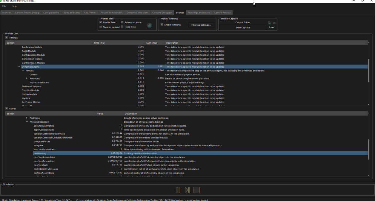
In order to see if the dynamics module is the bottleneck, enable the Timings option in the Profiler panel and examine the time spent by the DynamicsEngine in the Timings section by navigating to ApplicationUpdate > ModulesUpdate > DynamicsEngine.
For a breakdown of the time spent, enable the Values option and navigate to ApplicationUpdate > ModulesUpdate > DynamicsEngine > Physics > PhysicsBreakdown. The image below shows the detailed timings of the individual components in the physics engine pipeline.
High Time Consumption in "solveDynamics.computeForces"

Use the Solver Analytics panel to make the problem easier to solve
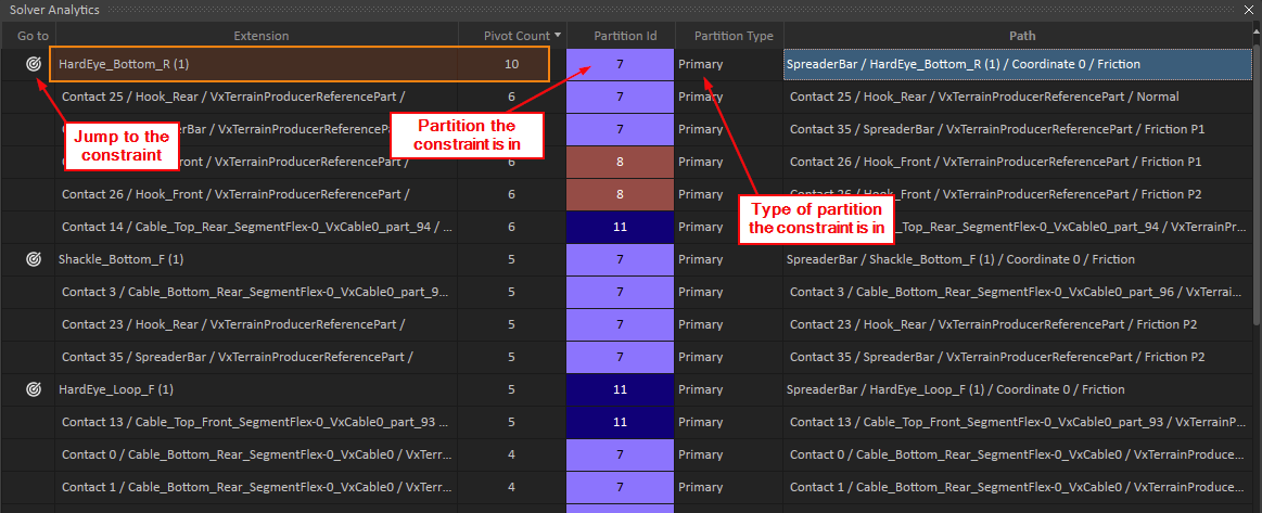
The solver could spend a lot of time to solve a stiff or overconstrained system. Some constraints could be relaxed, e.g., their stiffness reduced or their slip increased, in order to help the solver find a solution more quickly. In the Vortex Studio Editor, you can use the Solver Analytics panel to help you find the constraints that cause the slowdown and should be relaxed. The constraints that have a high pivot count are the ones that cause the most processing time in the solver.
Sorting the Solver Analytics panel's pivot count in decreasing order helpfully displays the worst offenders at the top. This allows the user to find the exact constraint rows (i.e., individual equations in the constraint) at the top of the list that slow the simulation down, as well as the rows that are harder to solve (the "stiff rows"). To help locate the offending rows, the Solver Analytics panel displays the extension that contains the constraint, its partition ID, partition type, and path. A button in the Go To column allows the user to easily navigate to the property view of the constraint in question.
|
| Example of a populated Solver Analytics panel |
|---|
Note that the constraint in this list was not necessarily created by the user. It could be a constraint created by dynamics extensions such as Vehicles, Tire Models, or Cables, or it comes from a contact, configured by the Material Table.
For relaxations of these kinds of constraints, the specialized interfaces of the corresponding dynamics extensions need to be used such as the Dynamics Properties extension in a Generic Cable. To navigate to the dynamics extension that is involved, use the Go To button on the left hand side in the Solver Analytics panel.
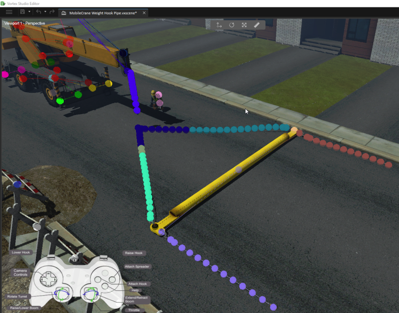
|
| Solver Analytics in the 3D View, using the same partition ID colors as displayed in the Solver Analytics panel |
|---|
To tune the simulation to reduce solver time consumption:
- Open the Solver Analytics panel.
- Sort the Pivot Count column from high to low.
- Navigate to the offending constraints at the top and either relax them, or remove or replace the corresponding constraints if they are redundant in the mechanism.
This procedure can be repeated until the pivot counts are consistently low in the simulation.
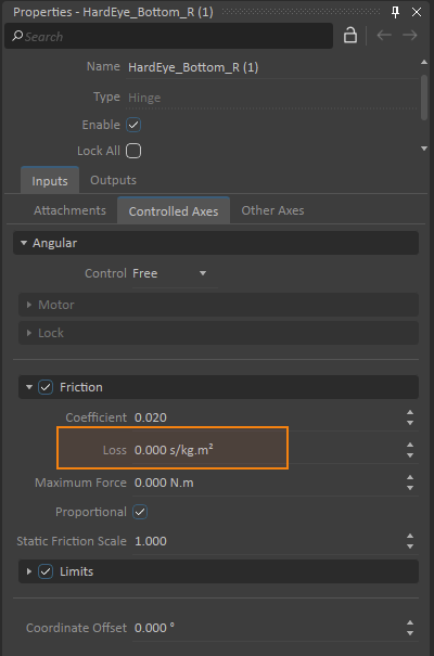
In the example seen in the screenshots above, the friction in coordinate 0 of the constraint "HardEye_Bottom_R" causes a relatively high pivot count of 10 pivots. Following the steps outlined above:
- Navigate to the constraint via the Go to button.
- In the constraint's Properties window, navigate to the parameters of the constraint row in question. In the example, this is the constraint's first coordinate ("Coordinate 0", as indicated in the Solver Analytics panel). For a hinge, this coordinate can be found in the Angular section of the Controlled Axes tab.
- Add some Loss in its Friction parameters. This will relax the constraint row and reduce the number of pivots required to solve for its force.
Split the problem and parallelize the work
Make sure that inactive simulation components can fall asleep
Use techniques to reduce time consumption when simulating long and detailed flexible cables
High Time Consumption in "collisionDetectionBroadPhase"
The first step in the physics pipeline is the broad phase. The broad phase computes the potential intersections between collision geometries. It is rarely the source of the bottleneck, but it can happen when a large number of collision geometries are present in the scene. A good way to improve the broad phase is to use composites for the collision geometries which are in the same part. At the broad phase level, all the collision geometries that would be in the same composite will be processed as only a single bounding volume. This will reduce the time consumption for the broad phase but will also have an impact on the contact generation. This impact is due to the so-called contact simplification process, which will consider the composite as a single collision geometry and will reduce the number of contacts accordingly.
Time Time Consumption in "collisionDetectionContactGeneration"
In the Profiler, under Physics > Census, Enabled Contacts reveals the number of available contacts. If the number is quite high, this could be the source of the performance problem. There are several ways to deal with this issue:
- Using collision rules can considerably reduce undesired or useless contacts.
- Using meshes with a high level of detail can be computationally expensive for the collision detection. You can try splitting your mesh into multiple convex meshes using the Convex Mesh Decomposition feature.
- Optimize the middle phase in the collision detection of your Terrain using the UV Grid Visualizer, which is an extension that help you to tune the terrain parameters.
- Many contacts are still enabled because rigid bodies are not sleeping. See Setting Sleep Thresholds of Parts for more information.
- An interaction between two rigid bodies generates too many contacts. By putting the collision geometries into a composite collision geometry, the number of contacts will be reduced via a process referred to as contact simplification.
Collisions with Deformable Terrains can cause high contact generation time consumption. Simplify the colliding collision shapes.
Colliding with a Deformable Terrain is very efficient, but deciding if it should be deformed plastically or permanently is not currently very efficient for complex parts. Parts such as vehicle wheels are very efficient, but deformer tools like blades, buckets, or complex shapes like a truck flatbed trailer are not as efficient.
You can design your parts to mitigate this. What follows here is a rough overview of the problem, and some possible solutions in content building.
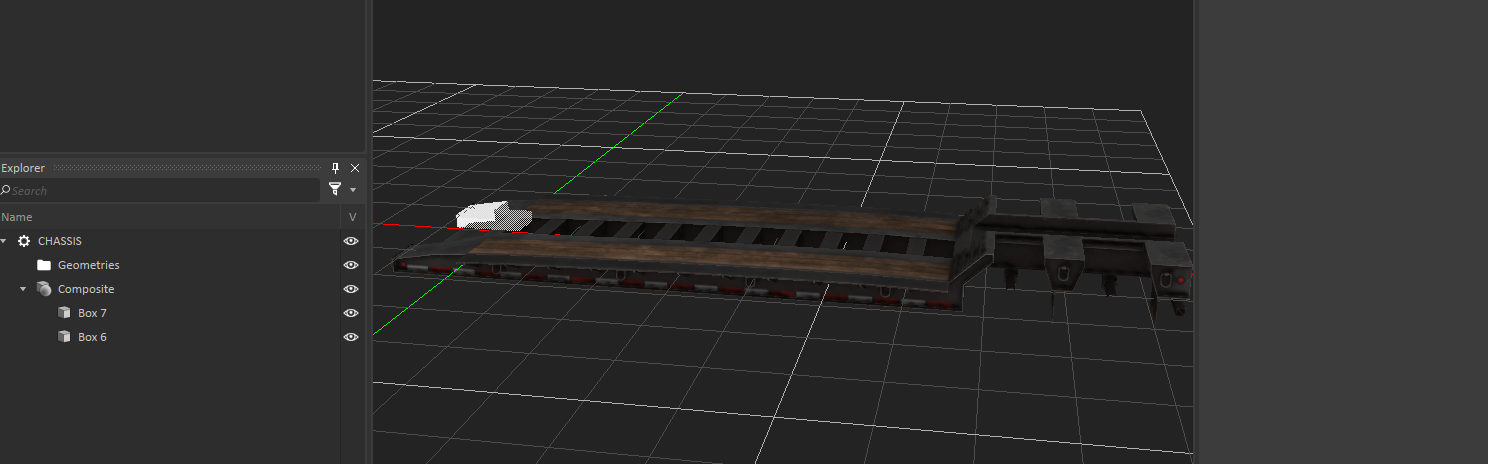
- In the example image below, the part has too many collision geometries.
- When simulated on a deformable terrain, the front section of the part has a high computation cost in ModulesPostUpdate > Earthwork Systems Module > SoilDynamics > SoilZoneTimings > SoilZoneTimingBreakdown > analyzePartFootprint.

- Simplify the model by:
- Reducing the number of collision geometries for dynamic parts in contact with deformable terrains
- Split off parts to achieve the same result and constrain the new part to the original part
- When simulated on a deformable terrain, the front section of the part has no more computation cost than the rear section.
- In the example image below, the part has too many collision geometries.
High Time Consumption in "stepExtensions"
Fluid Interaction
Using fluid interaction is likely the source of this problem. If a lot of rigid bodies or complex triangle meshes are used in a fluid, that could be the cause of your slowdown in performance. Simplifying your fluid collision geometries can solve this issue.
Earthwork Systems
Earthwork systems simulations could be the cause of the issue. Using a larger cell size for Earthwork Zones and Soil Bins could be a solution to this performance problem.
To confirm that the soil particle simulation is the cause of the slowdown, consult the detailed soil dynamics timings under ModulesPostUpdate > Earthwork Systems Module > SoilDynamics.
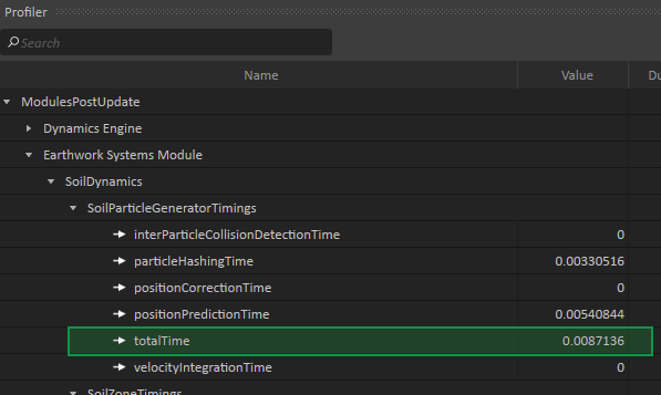
Note that the displayed timing measurements are in milliseconds. For more potential performance issues in soil simulation, consult Finding Bottlenecks in Earthwork Simulations.
Custom Extensions
If you have written your own IDynamics extension, your code could be the source of the issue.
High Time Consumption in "intersectSubscribers"
This could be related to an intense use of sensors and triggers.
Alternatively, if you wrote an extension which uses an implementation of the class VxUniverse::IntersectSubscriber, it is possible that the time is spent in this implementation.
Finding Bottlenecks in Earthwork Simulations
Additional, specialized simulation components are used in Earthwork Systems. These simulation components are enabled by adding the Earthwork Systems module to your Application Setup (.vxc) file. For the purpose of tracking time consumption of these components, the Earthwork Systems module exposes additional, focused timing measurements ranging from soil particle simulation time to the time it takes to simulate soil erosion on the diggable soil zones. This profiling information can be found in the Profiler under ModulesPostUpdate > Earthwork Systems Module > SoilDynamics, as seen below.
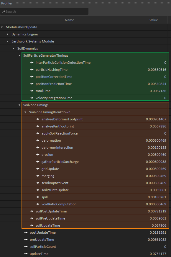
The measurements are grouped in "time spent on soil particle simulation" (highlighted in green in the screenshot) and "time spent on updating the diggable soil zones" (highlighted in orange). The displayed values are given in milliseconds.
If the time consumption of certain simulation components from this list become too high, certain remedies can be applied to reduce the workload and speed up the simulation. Below is a list of common bottlenecks and the corresponding solutions.
High Time Consumption in "SoilParticleGeneratorTimings > totalTime"
This case indicates that there are probably too many particles in the simulation for the simulation to run smoothly on the given hardware. The soil particle simulation is parallelized and can be sped up by using faster processors with more cores. If this is not an option, you can either limit the number of particles via the Soil Materials Extension, or use smaller particle sizes.
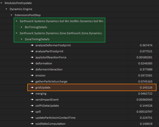
High Time Consumption in "SoilZoneTimings > SoilZoneTimingsBreakdown > gridUpdate"
This likely indicates that an Earthwork Zone in the simulation is rather large and has the Output Mass parameter selected. If possible, deselect Output Mass; this will eliminate the bottleneck in gridUpdate. At the same time, this will no longer provide the mass of the Earthwork Zone as an output field. As an alternative, use a Soil Mass Sensor to measure the mass in a smaller area of interest. Otherwise, the cell size of the Earthwork Zone or Soil Bin which is the cause of the bottleneck can be reduced to lower the time consumption. In order to find the Earthwork Zone or the Soil Bin which is causing the slow down, it is possible to consult detailed timings per zone or bin. These timings can be found under the post update timings of the dynamics module as shown below.
High Time Consumption in "updateParticlesInContactTime" (of a specific Earthwork Zone or Soil Bin)
It is possible that significant time is spent to produce the list of particles which are traveling on an Earthwork Zone or a Soil Bin. This bottleneck can be identified by inspecting the detailed timings of the individual zones or bins as shown below.
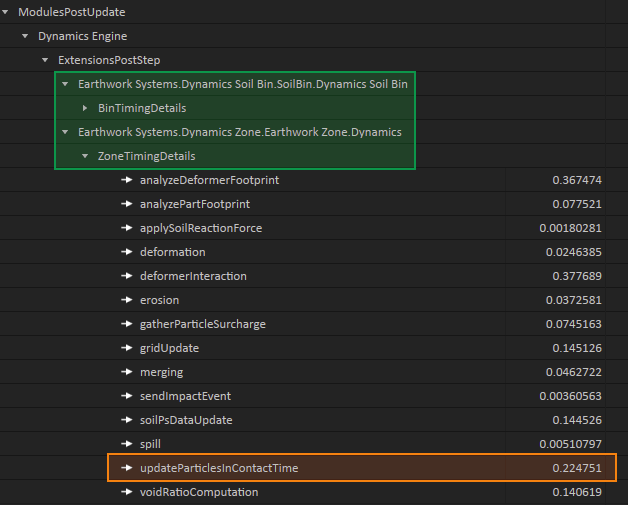
If the updateParticlesInContactTime is found to be elevated, the Output Particles parameter on the corresponding zone or bin can be deselected to disable the calculation of this particle list. This will completely remove the time spent. The consequence of this modification is that the particles traveling on the corresponding soil surface can no longer be wrapped by the graphical height field. This is not an issue if the Screen Space Mesh option in the Soil Particles Extension is used for displaying simulated soil particles.